The USGS topo maps are awesome … especially when using them for the outdoors or doing historical research.
The maps contain a great deal of information on public lands, national parks, nature preserves and most other United States public lands
The highlighted features include: trails, amenities, ranger stations, boundaries, elevation data, bathymetry, roads, contour lines, and hill shading, etc.
Even better the USGS has topo maps going all the way back to the year 1882. 🤩
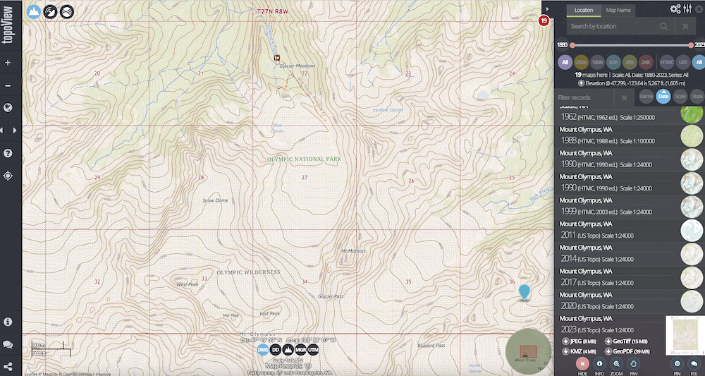
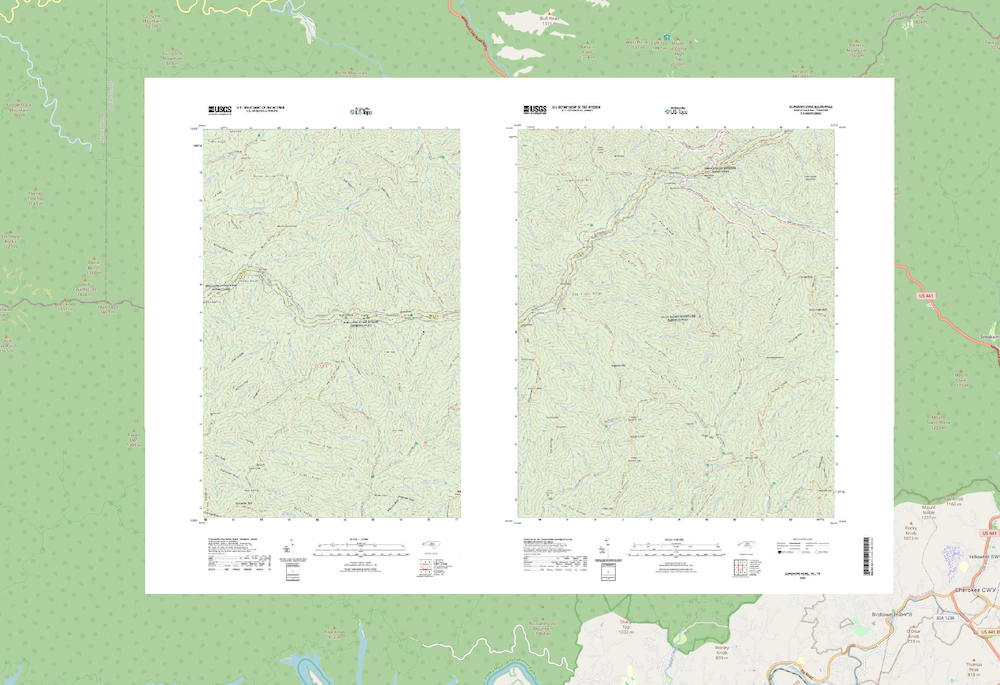
Here is an example of what the latest year 2023 USGS topo map looks like for Mt. Olympus when viewed on topoView.
Overview
- Background
- Goals
- Prep Work
- Download USGS GeoPDFs
- Convert to GeoTiffs
- Clip Collars
- Creating Map Tiles
- Creating PMTiles
- Upload PMTiles to S3
- Results
- Lessons Learned
- Why?
- Next Steps
Background
If we wanted to use these maps in our own app or as map tiles we have some issues:
- topoView is an application from the USGS where you can pan around and download 7.5 minute quadrangles in JPEG, GeoTiff, KMZ, or GeoPDF. ⚠️ However, you have to download individual images, GeoPDFs, or GeoTiffs.
- topoBuilder is a marketplace of sorts where you can select a 7.5 minute quadrangle or 100K topo and they will email it to you. ⚠️ Email doesn’t work at scale and is definitely not a mosaic.
- National Map this map is a tad different style than the normal USGS topos… not sure why, but nonetheless it is a neat map, but some issues:
- They do have an ArcGIS endpoint, but I don’t want to depend on someone else’s API that is free and could change anytime.
- Their tile server seems pretty slow.
- I’m not sure their usage policy for offline / bulk downloads from their ArcGIS services.
- The maps GeoTiffs/GeoPDFs have collars around them by default which means if you tried to directly place them together there would be whitespace around them like this when viewed in QGIS: 🤮

Goals
So what are we going to do then?
- Make a seamless mosaic USGS topo map with the latest map from each 7.5 quadrangle.
- Self host the map tiles with Protomaps.
- Add this base map to Topo Lock Maps.
- Have fun making maps, working with raster data, GDAL, Rasterio, and doing data engineering stuff.
Let’s get started.
“If you spend too much time thinking about a thing, you’ll never get it done.” -Bruce Lee
Prep Work
There are ~65,000 7.5 minute quadrangles that compose the entire continental US, Alaska, Hawaii, Virgin Islands, and Puerto Rico.
Downloading all of the USGS quadrangles, including temporary storage takes up nearly 4 TB of space.
I spoke to my good buddy Seth who is hardware guru and I specified the data I’m working with and what all is involved. Since it is going to be a crap ton of reads and writes and we want the best performance I went with a 4TB M.2 NVMe drive and external enclosure for SPEED! 💾 🚀
- M.2 NVMe: WD Black SN850X NVMe
- Enclosure: Acasis 40Gbps M.2 NVMe USB 4 Thunderbolt 3/4 SSD
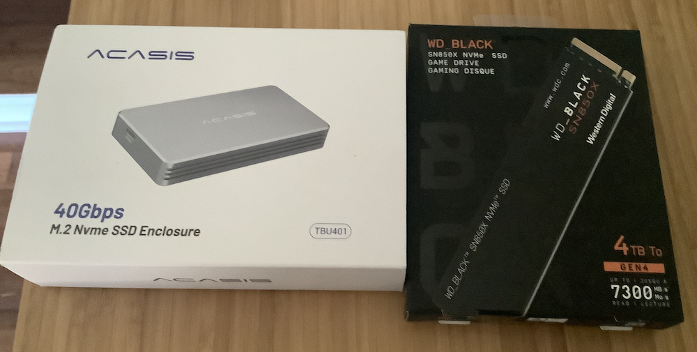
I formatted the drive with APFS because I have had a lot of good success dealing with large files on APFS.
See this X conversation with me and @shademap discussing drive formats… basically, choose your drive format wisely.
Download USGS GeoPDFs
Let’s scrape all of the appropriate US Topo GeoPDFs quadrangles from AWS S3. There are ~65,241 of them!
The USGS topo maps can be found on this s3 bucket.
Example script for Alaska:
| |
I downloaded every single current USGS topo GeoPDF and put them on a folder on my NVMe drive.
Convert to GeoTiffs
The great thing about downloading GeoPDFs is we can selectively enable and disable individual layers when converting to GeoTiffs.
💡 We can use this in the future for building different versions of the map; for example maybe we wouldn’t want a map with hill shading or contour lines, or maybe just aerial imagery only.
So let’s figure out which layers we want on this version of the map.
Let’s take an example of NC_Clingmans_Dome_20220916_TM_geo.pdf.
We can view each GeoPDFs layer by using GDAL, and the parts we are specifically looking for right now is under the Metadata (LAYERS): section:
| |
We have 26 layers:
| |
To quickly test how the map will look with different layers enabled/disabled, open the GeoPDF with a PDF viewer.
For example, here is an example of what it looks like when opening NC_Clingmans_Dome_20220916_TM_geo.pdf with the standard Acrobat Reader on macOS:
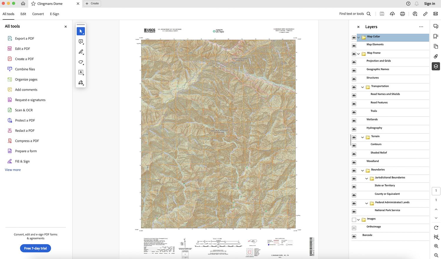
As you can see on the right side most of the layers are enabled in this particular GeoPDF.
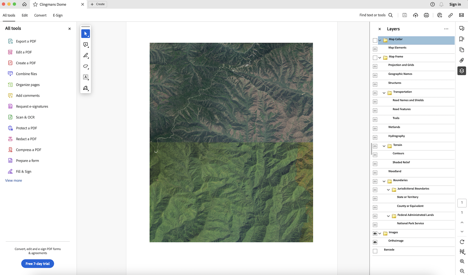
For example, if we disable everything except for Orthoimage, this is what we will see (only aerial imagery):
So now it’s time to code because we need to automate all this!
| |
This gdalwarp command does the following:
- Line 2 -
t_srs EPSG:3857- Reproject/transform SRS toEPSG:3857 - Line 3 -
COMPRESS=JPEG- Set compression to JPEG, I found this to be the best balance of quality vs. size of the tiles - Line 4 -
PHOTOMETRIC=YCBCR- I read Paul Ramsey’s post about GeoTiff Compression for Dummies. - Line 5 -
TILED=YES- It’s a best practice to set this for performance reasons documented on the GeoTiff driver - Line 6 -
QUALITY=50- I played around with different quality settings and this greatly reduces the storage size of the resulting tiffs with very minimal impact to quality. Paul Ramsey’s post about GeoTiff Compression for Dummies talks about this too. - Line 7 -
of GTiff- Output to a GeoTiff - Line 8 -
GDAL_CACHEMAX 1000- Set the GDAL block cache size, read about it here. - Line 9 -
GDAL_NUM_THREADS "ALL_CPUS"- speeeeeed 🚀 - Line 10 -
GDAL_PDF_LAYERS "ALL"- Turn on all PDF Layers first, see I needed to do this below. - Line 11 -
GDAL_PDF_LAYERS_OFF- Turn off PDF layers we don’t want - Line 12 -
GDAL_PDF_DPI 300- Set GDAL DPI to 300
⚠️ The reason for using both GDAL_PDF_LAYERS and GDAL_PDF_LAYERS_OFF is I found out I needed to enable all the layers first, then selectively disable the ones I didn’t want. The reason is because some of the GeoPDFs have different settings “saved” internally so if we just disable then we will get mixed results when creating a mosaic.
I put this entire script in a python script and ran it in a loop:
| |
✅ Now we have all 65,000+ GeoTiffs reprojected, compressed, with only the layers we want.
🔥 This part of the process on my mac M2 Max 95 GB RAM took 40 hours and ~300 GB of GeoTiffs.
| |
Clip Collars
These pesky collars! There is so much discussion around the Internet on the best way to remove the collars from around individual 7.5 minute quadrangles.
Let’s use Rasterio to clip / mask the USGS topo map collars:
- The USGS maintains the 7.5 Minute Map Indices: https://prd-tnm.s3.amazonaws.com/index.html?prefix=StagedProducts/MapIndices/National/GDB/
- Read the the map indices geopackage with GeoPandas:
1 2 3 4national_7_5_minute_indices = geopandas.read_file( DATA_DIRECTORY / "MapIndices_National_GDB.gdb/", layer="CellGrid_7_5Minute") national_7_5_minute_indices = national_7_5_minute_indices.to_crs('EPSG:3857') - For each GeoTiff get the centroid:
1 2 3 4 5 6 7 8 9 10 11def get_geo_tiff_centroid_point(geo_tiff): transform = geo_tiff.transform crs = geo_tiff.crs width = geo_tiff.width height = geo_tiff.height middle_x = width // 2 middle_y = height // 2 # Convert middle pixel indices to coordinates lon, lat = transform * (middle_x, middle_y) centroidOfTif = Point(lon, lat) return centroidOfTif - For each centroid of the GeoTiff, do a spacial join and find the corresponding quadrangle geometry and mask the GeoTiff to that using Rasterio:
1 2 3 4 5 6 7 8 9 10 11 12 13 14 15 16 17 18 19 20 21 22 23 24 25 26 27 28 29 30 31 32def mask_geo_tiff(geo_tiff_file_name): geo_tiff = rasterio.open(geo_tiff_file_name) centroid = get_geo_tiff_centroid_point(geo_tiff) centroidSeries = geopandas.GeoSeries([centroid], crs='EPSG:3857') centroidDataFrame = geopandas.GeoDataFrame({ 'geometry': centroidSeries }, crs='EPSG:3857') assert national_7_5_minute_indices.crs == centroidDataFrame.crs indices_join = national_7_5_minute_indices.sjoin( centroidDataFrame, how="inner", predicate="contains" ) shapes = [indices_join["geometry"] for r in indices_join] shape = shapes[0] filext = ".mask.tif" #https://rasterio.readthedocs.io/en/stable/topics/masking-by-shapefile.html with rasterio.open(geo_tiff_file_name, crs=dst_crs) as src: out_image, out_transform = rasterio.mask.mask(src, shape, nodata=255, crop=True) out_meta = src.meta out_meta.update({"driver": "GTiff", "height": out_image.shape[1], "width": out_image.shape[2], "transform": out_transform}) with rasterio.open(f"{geo_tiff_file_name}{filext}", "w", **out_meta, compress="JPEG", tiled=True, blockxsize=256, blockysize=256, photometric="YCBCR", JPEG_QUALITY=50) as dest: dest.write(out_image)
The key part of this process is using Rasterio masks:
- I’m setting the nodata value to white
nodata=255so that the seams of the mosaic are white instead of black. This looks much better with a mosaic so you can’t see the seams as much once the final map is all together. Below is an example of the seam where you can see where the quadrangles fit together: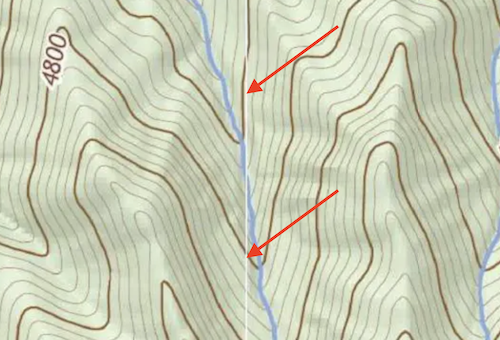
- Good reading material on masking with Rasterio:
Here is an example of what the GeoTiffs look like with and without collars:
| With Collars | Without Collars |
|---|---|
 |  |
Results so far:
- At this point we now have all of the 65,000+ USGS GeoTiffs, reprojected, collars clipped, and ready to make some map tiles!
Creating Map Tiles
I did a lot of testing with different tools to see what performed best and created the best looking tiles.
A few things we need to deal with:
- The USGS topos are not contiguous since it is only for the US and especially around the coastline there are quadrangles that the USGS does not provide. Therefore, we don’t want to write black opaque tiles in those places because that would take up unnecessary space and it looks bad. WEBP transparency will help here.
- We will need a GDAL virtual dataset, however building a GDAL virtual dataset with 65,000+ files won’t work with the standard command of
gdalbuildvrt -addalpha all.vrt *.tif.- Instead we will need a script to build the virtual dataset. Create a file named
build-vrt.shand add the following to it:1 2 3 4 5 6 7 8 9 10 11 12 13 14 15 16 17 18 19 20 21 22 23 24 25 26 27rm allfiles.txt ls A*.tif >> allfiles.txt ls B*.tif >> allfiles.txt ls C*.tif >> allfiles.txt ls D*.tif >> allfiles.txt ls E*.tif >> allfiles.txt ls F*.tif >> allfiles.txt ls G*.tif >> allfiles.txt ls H*.tif >> allfiles.txt ls I*.tif >> allfiles.txt ls J*.tif >> allfiles.txt ls K*.tif >> allfiles.txt ls L*.tif >> allfiles.txt ls M*.tif >> allfiles.txt ls N*.tif >> allfiles.txt ls O*.tif >> allfiles.txt ls P*.tif >> allfiles.txt ls Q*.tif >> allfiles.txt ls R*.tif >> allfiles.txt ls S*.tif >> allfiles.txt ls T*.tif >> allfiles.txt ls U*.tif >> allfiles.txt ls V*.tif >> allfiles.txt ls W*.tif >> allfiles.txt ls X*.tif >> allfiles.txt ls Y*.tif >> allfiles.txt ls Z*.tif >> allfiles.txt - Run
build-vrt.sh - Now we can run
gdalbuildvrt -addalpha all.vrt -input_file_list allfiles.txtwhich will work with 65,000+ files. - We want to use the option
-addalphaso that tiles with no data we have alpha since we are making WEBP tiles. You can read more about that on the docs.
- Instead we will need a script to build the virtual dataset. Create a file named
Tiling Options:
I did a bunch of testing with what would be the best performance that gives us WEBP tiles. This video from FOSS4G 2023 Tiling big piles of raster data using open source software and MapTiler Engine has a pretty good overview of the situation.
We want to stay open source so I’m going to try:
- gdal2tiles.py
gdal2tiles_parallel.py- gdal_translate & gdaladdo
✅ First Option: gdal2tiles.py:
1 2 3 4 5 6 7 8 9gdal2tiles.py \ --exclude \ --tilesize=512 \ --processes=12 \ --tiledriver=WEBP \ --resampling=bilinear \ --zoom="0-15" \ --xyz \ all.vrt tiles- ⭐ This is the option I have decided to go with for now and works pretty well.
- It creates a directory of XYZ tiles.
- It output some weird
webp.aux.xmlfiles.- I’m not sure what the heck these things are. But I figured it might hurt performance if I don’t need them and gdal2tiles is having to write them.
- It seems like these are for ArcGIS or something? I dunno. You can read about them here.
- I turned them off by running:
1export GDAL_PAM_ENABLED=NO
- Since this outputs XYZ tiles we need to package them up in mbtiles:
- Install mb-util
- Add the metadata.json to the root of the tiles folder that is used by mb-util
1 2 3 4 5 6 7{ "name": "USGS 2024 Current Topo Maps", "description": "USGS Topo Maps", "version": "1", "minzoom": 0, "maxzoom": 15 } - Package .mbtiles:
1 2 3 4 5mb-util \ --silent \ --scheme=xyz \ --image_format=webp \ input_tile_folder out.mbtiles
🚫 Second Option:
gdal2tiles_parallel.py:- ❓ This seems like an old script that was put together and I’m not sure if at some point this was merged into GDAL.
- ❓ There are several variations and versions floating around on Github.
- 🚀 This was the fastest I tried.
- ⛔ Does not support WEBP.
🚫 Third Option
gdal_translate&gdaladdo:- 🦥 This option is VERY VERY slow. Like sloth slow. I let this run overnight one night trying to process all GeoTiffs and it never even reached 1% done.
- ⛔ Does not look multi threaded
- ⛔ Does not support WEBP
- ⛔ Have to separately run
gdaladdoaftergdal_translatewhich takes additional processing time. - Sample Commands I tried:
gdal_translate --config GDAL_NUM_THREADS ALL_CPUS --config GDAL_CACHEMAX 25% -of MBTILES -co TILE_FORMAT=JPEG -co QUALITY=50 -co BLOCKSIZE=512 all.vrt output.mbtilesgdaladdo -r average output-gdaladdo-average.mbtiles --config COMPRESS_OVERVIEW JPEG --config JPEG_QUALITY_OVERVIEW 50 --config PHOTOMETRIC_OVERVIEW YCBCR --config GDAL_NUM_THREADS ALL_CPUS --config GDAL_CACHEMAX 75% --config GDAL_TIFF_OVR_BLOCKSIZE 512
💯 So at this point, we have used mb-util to package the tiles into .mbtiles, from the XYZ tiles generated from gdal2tiles.py, that were generated from the GeoTiffs that we extracted, clipped, and reprojected from the GeoPDFs. Whew. 😅
The hard part is done.
Creating PMTiles
Using the protomaps go library we can convert our mbtiles to pmtiles!
Let’s see how fast we can convert 300 GB of mbtiles:
% time ./pmtiles convert usgs-topo-2024.mbtiles usgs-topo-2024.pmtiles
2024/02/29 22:41:06 convert.go:260: Pass 1: Assembling TileID set
2024/02/29 22:41:10 convert.go:291: Pass 2: writing tiles
100% |████████████████████████████████████████████████████████████████████████████████████████████████████████████████| (20332169/20332169, 5866 it/s)
2024/02/29 23:38:56 convert.go:345: # of addressed tiles:  20332169
2024/02/29 23:38:56 convert.go:346: # of tile entries (after RLE):  19768407
2024/02/29 23:38:56 convert.go:347: # of tile contents:  19594193
2024/02/29 23:38:59 convert.go:362: Root dir bytes:  9385
2024/02/29 23:38:59 convert.go:363: Leaves dir bytes:  42486391
2024/02/29 23:38:59 convert.go:364: Num leaf dirs:  3501
2024/02/29 23:38:59 convert.go:365: Total dir bytes:  42495776
2024/02/29 23:38:59 convert.go:366: Average leaf dir bytes:  12135
2024/02/29 23:38:59 convert.go:367: Average bytes per addressed tile: 2.09
2024/02/29 23:41:09 convert.go:340: Finished in  1h0m3.023499209s
./pmtiles convert usgs-topo-2024.mbtiles usgs-topo-2024.pmtiles
    572.24s user 611.80s system 32% cpu 1:00:03.89 total
⭐ Only 1 hour! Protomaps and pmtiles are just so good. Protomaps is totally going to change the mapping landscape long term!
This results in a 300 GB .pmtiles file!
Upload PMTiles to S3
Using the same protomaps go library we can upload our pmtiles to our s3 bucket:
export AWS_ACCESS_KEY_ID=GET_YOUR_OWN_KEY
export AWS_SECRET_ACCESS_KEY=GET_YOUR_OWN_KEY
export AWS_REGION=us-east-2
./pmtiles upload usgstopo.pmtiles usgstopo.pmtiles --bucket=s3://some-awesome-bucket
My home Internet upload speed is terrible, so I had 👍 my friend Jason upload it for me. So yes, I shipped him an encrypted SSD with the pmtiles 🤣
Results
This is what the resulting mosaic USGS topo map looks like zoomed out to include the continental US, Alaska, Hawaii, Puerto Rico, and Virgin Islands:
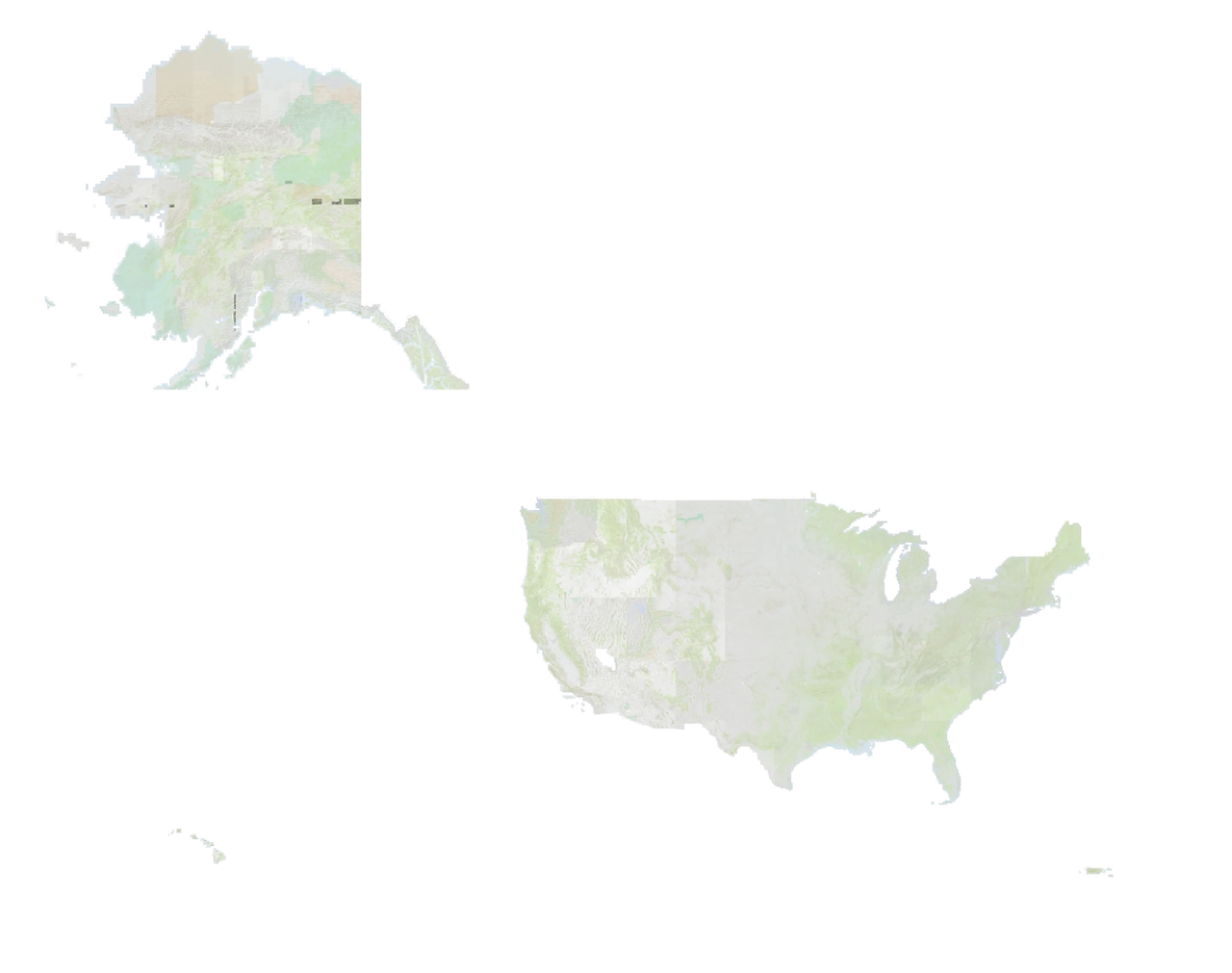
I have also included this map in Topo Lock Maps!
Lessons Learned
The entire process in the end is: GeoPDFs > GeoTiffs > Masked GeoTiffs > .mbtiles > .pmtiles > great success
- 💪 This was my first time processing this much raster data on my local machine and it was a huge challenge… glad I pushed through because the map looks amazing!
- 💾 Always process large geospatial data on an external drive, preferably an NVMe because there is a lot of reading and writing of files/tiles and you can get huge performance boosts from an NVMe rather than an SSD.
- 🚀 Ensure your NVMe drive is an appropriate disk format for very large files. I went with APFS. See this X conversation with me and @shademap discussing drive formats… basically, choose your drive format wisely.
- 👌 Along the way I ran a data quality checks to ensure I had every single quadrangle and there were no missing quadrangle holes… I wanted a seamless mosaic!
- I iterated each of GeoPDFs using Python & GeoPandas. For each GeoPDF get the centroid and write the centroids to a dataframe.
- Take the entire 7.5 minute USGS Grid Geopackage and using all the centroids from the GeoPDFs, I found any missing GeoPDFs.
- This proved useful because during the initial download of the GeoPDFs some of the downloads did not finish even though I never saw any errors in my terminal.
- 😱 One night while I was creating mbtiles of the continental U.S., I filled up my entire macOS internal SSD because I accidentally created the tiles on my internal macOS SSD rather than my external NVMe. 😠 My mac was unresponsive and I had to boot into safe mode. I couldn’t even do a
rm -rfon files because how APFS works. Disk util said I had 3.6 MB free. Crap. I couldn’t even delete Time Machine snapshots. I tried to go down the path of deleting the recovery volume. But end the end, one night I had to just sit there, in the macOS system restore terminal and copy off the temporary tile data that I had just created over the last 24 hours to my external NVMe. The copy took hours because of all the hundreds of millions of WEBP tiles 🤣. What a crazy event. Good thing I had Time Machine backups for my entire laptop for my normal day-to-day business data.
Why?
Some people ask why self host maps and instead just directly point to the USGS data and use something like STAC?
Mostly because it is fun and I’m crazy, but there are other reasons too.
So the issue for me is if I point Topo Lock Maps directly to a someone else’s API that I don’t have control over then I have to deal with situations like:
- What if the underlying data changes?
- What if the underlying data is deleted?
- How often is the data updated?
- What if the performance degrades?
- Do they support bulk downloads?
- Or other unknown unknowns
Kyle Barron played around with doing this with COGs.
Now if I’m paying for a service / API / data and there is a contract and licensing terms, then that is a different story, but in this situation this public free data with no guarantees.
So I can’t risk that.
In order to make the best possible experience in Topo Lock Maps I’m trying to self host so I have full control over the API, data, and privacy considerations.
Next Steps
I actually have all this running in Dagster and automated so I can keep the map updated in Topo Lock Maps so I can materialize a USGS topo pmtiles file all with a single button click!
So maybe I’ll write about data engineering and orchestration on down the road.
🤝 Huge thanks to the USGS for making such great maps!
🤝 Thanks to Seth for hardware knowledge.
🤝 Thanks to Jason for his Internet.
🤝 Thanks to protomaps for being freaking awesome.
“Do not pray for an easy life, pray for the strength to endure a difficult one.” -Bruce Lee